Avoiding #INVALID DATA TYPE when cells are blank

Hello,

I am setting up a staffing leave Smartsheet for my team and unfortunately I am getting the #INVALID DATA TYPE error message.

There are 2 formulae set up within the sheet:

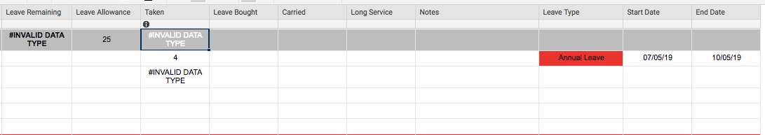
Leave Remaining (the dark grey row) is calculated as follows: =[Leave Allowance] - Taken + [Leave Bought] + Carried + [Long Service]

Taken (the dark grey row) is calculated as follows: =SUMIFS(Taken2:Taken6, [Leave Type]2:[Leave Type]6, "Annual Leave") - There are other types of leave but for this instance I only want it to calculate annual leave.

I realise the error message is coming up as there is no data in the start date/end date on row 3 however, how can I get round this. In Excel, it would allow me to have no data in and it would fill the Taken column with a value of "0".

Is it a different formula I need to apply? Any help would be much appreciated!

Screenshot 2019-04-11 12.28.32.png

Find more posts tagged with

Human Resources

Sheets

Formulas

Solution Center

Media & Entertainment

Comments

L_123

What you are talking about is the iferror formula:

=iferror([Leave Allowance]@row- Taken@row + [Leave Bought]@row+ Carried@row + [Long Service]@row),0)

you can switch the 0 to "" if you want to make it blank if there is an error.

That said, If error is not what you need. If the cell is blank, your formula should treat it as a 0. That said your leave remaining formula is referencing taken1 which has an error. taken1 is referencing taken3 which has an error. That means that taken3 is causing both the other errors. if you delete what is in cell taken3 the errors should go away.

Also, you need to add row references to your leave remaining formula. you can either do @row, or just put a 1 there, but it won't reference anything without a row reference.

SteCoxy

Thank you kindly for taking the time to reply to my query.

I've got to be 100% honest I am a total novice with formulas in spreadsheets, so I'm slightly confused by your response sorry! Any chance you could explain in layman's terms?

Ideally what I am wishing for is the cell in "Taken" column to either be blank or show a zero until I enter dates in the "Start Date" and "End Date" columns but at present when I try and apply the formula in this cell the error message is coming up, which then affects the dark grey row for both "Leave Remaining" and "Taken".

Mike Wilday

All of those errors are being created by the formula in Taken3. What formula are you using in Taken3?

Try using this formula in row 3 of the taken column.

=IFERROR(Networkdays(Start@row, Finish@row),"")

SteCoxy

In Taken3 I am using the following formula: =NETWORKDAYS([Start Date]3, [End Date]3)

Mike Wilday

Try plugging the formula I shared. the @row replaces the row number and searches the row you have the formula in. Plug that formula in and see if it works for you. =IFERROR(Networkdays(Start@row, Finish@row),"")

That formula will leave the cell blank when there isn't a start or a finish date.

Amy Shank

I believed I've fixed the formula to correct the @cell invalid data type error and instead it returns a blank cell. However, I've used the following formulas to try and get the average from a column in my spreadsheet but I keep getting an invalid data type error in the sheet summary formula..

=AVG([LE Total Days]:[LE Total Days])

=AVG(COLLECT([LE Total Days]:[LE Total Days]), ISNUMBER,(@cell)))

Sign in to join the conversation!

Quick Links

Trending discussions

Getting error message in approval email
Hey, Is anyone else facing this issue in the approval notifications sent through smartsheet
Add Package Count Based on Customer
I have a sheet with a list of customers in one column, and then the following columns are City, Monday, Tuesday, Wednesday, Thursday, Friday. I need help with a formula that I can put in my sheet summary so that if the customer column says Staples (It can say this in multiple rows) that it will tell me the total package…
Automation not triggering all of the time
Hi Smartsheet community, I've always tried to answer questions but this is my first time posting. So I have formula =IF([Project Status]@row = "Complete", 1, 0) set up in the "Complete Check - Hide column" to check the box when the project status is marked complete. The project status column is tied to several other sheets…