How to return specific Column from a Multi Column Cross Sheet Range

Huntb2000

Hi Folks,

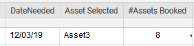
I have the following formula used to track specific assets:

=SUMIF({EventDate_req}, $DateNeeded$1, {Asset2_Range})

This adds up the count in each row in the Asset2_Range that matches the date needed.

We created individual one column ranges for each asset (Asset1, Asset2, Asset3) etc.

Problem is we are using too many cross sheet references and need to replace each of these 1 column wide ranges with one range that has all the columns and then use an index (like we would with vlookup to select which column we want to check.

So if I create one range Called ALL_Assets_Range that has side by side columns Asset1, Asset2, Asset3.

Question is:

How do I update the formula above to point to the first column or the second column of this now multi column range?

For example to look up Asset2 it would be something like

=SUMIF({EventDate_req}, $DateNeeded$1, {ALL_Assets_Range[2]})

How do I accomplish the goal of making the last parameter return all values from the specific column of the multi column range??

The sheet is getting very slow so would appreciate any help on this formula and ways to speed up.

Thanks!

Find more posts tagged with

Formulas

Cell linking

Comments

Barry Bowles

Hi there - I'm a little unsure of what result you are looking to generate. Are you looking to get a different total count for each Asset or a combined total count of all Assets that match the date?

Huntb2000

Hi Barry,

the goal is sum up all assets in that Asset column that match the date in the event date column.

The current setup has a 1 column wide cross sheet range for each asset that is used to sum up based on the date.

We want the same result - how many of asset 1 are needed for a specific date, created by adding up each Asset number in each row of that asset that match the date in that row to the target date

Each row in the sheet is for an event

There is a date column for each event

Each event can select 1 or more of the assets in each asset column.

The current formula works but as mentioned, uses a range that is only one column wide.

We want to create one range that is multi column. then in the formula we want to specific which relative column number (in that cross sheet range) we want to use to add up - essentially selecting a specific resource by using the column number in that range that represents the asset we want to count.

Thanks for looking into this for us!

Huntb2000

To be clear

this formula is run from a Summary Sheet and points to the asset sheet with ranges.

Current formula that works:

SUMIF({EventDate_req}, $DateNeeded$1, {Asset2_Range})

{EventDate_Req} is the date column for each event in the asset sheet

{Asset2_Range} is the Asset2 Column (for that specific asset) in the asset sheet

$DateNeeded$1 is the date in the Summary Sheet we want to use for the sum and when we get the total it is displayed next to that resource name in the summary sheet.

Barry Bowles

Hi again - thanks for the additional notes on what you are doing. It sounds like you want to populate more than one cell in your summary sheet with a single formula - is that the case? It might help if you showed me the structure of your summary sheet (remove any confidential data). My "picture" of your Asset sheet is a single column for each Asset containing the EventDates that Asset is needed for - do I have that picture right?

e.g.

Asset1 Asset2 Asset3 etc

eventDateReq1 eventDateReq1

eventDateReq2 eventDateReq2

eventDateReq3 eventDateReq3

eventDateReq4

etc

Huntb2000

Thanks Barry,

The issue is not more than one thing in the summary. There is no problem with the summary - The question here is on one thing only and that is how to sumif on a range and be able to specify which column in that range to use when summing.

Here is more details with an example:,

The Asset table is where I need the help:

Event EDate Asset1 Asset2 Asset3

ABC 12/3/19 3 1 5

QRS 12/1/19 8 7 1

XYZ 12/3/19 1 2 3

The current formula in the summary has a range for the EDate and a seperate range for each asset column.

So If I say SUMIF({EventDate_req}, 12/3/19, {Asset2_Range})

Where {EventDate_req} is the range for the EDate column above

{Asset2_Range} is the range for the Asset2 column above.

It will correctly return 3 since there are two events on 12/3/19, one needing 1 and one needing 2

Goal is to replace the three individual asset ranges with one Multi-column range called Asset_All that has all three columns in it.

When that happens how can I do the sumif on Asset_All just like I do it for Asset2?

How do I tell the sumif that the set of cells to sum out of the asset range will be only the ones in Column 2 (since Asset2 would be the 2nd column in the 3 column range? I will know it is Column 2 so I can put the 2 where it is needed in the formula.

So it would logically be something like this

SUMIF({EventDate_req}, 12/3/19, {Asset_All[2]) if [2] could be used to specific column #

that would simply mean use column 2 out of Asset_All in the formula - this is what I need to find out - how to tell smartsheet formula which column to use in a multi column range.

Thanks again for looking into this.

Barry Bowles

OK Thanks - that clarified the range on Asset sheet. I have a solution but it really depends on how many Assets you have - your example only uses 3 and my solution uses nested IF statements so it will be OK for a relatively small number of Assets but if there is more than about 8 to 10 Assets I would suggest the use of a lookup table for the Assets with each Asset proving the range reference to the formula via a vlookup statement

Here's my formula

=SUMIF({EDate}, DateNeeded1, IF([Asset Selected]1 = "Asset1", {Asset1}, IF([Asset Selected]1 = "Asset2", {Asset2}, {Asset3})))

I created a simple summary sheet that has a column to input the date needed "DateNeeded1"and a column to select the Asset from a drop-down list [Asset Selected]1 So you select the required Asset from the drop-down list and the formula sums the appropriate Asset column see attached screenshot

I hope this does the trick for you.

Paul Newcome

The best way to accomplish this would be to pull the data on the source sheet and then use cell linking to move it to the master sheet.

The absolute easiest way to do this would be to create a new row at the top of your sheet and then indent every row underneath of it. you can then use

=SUM(CHILDREN())

Across all columns of that one parent row to collect your data then link that parent row to your metrics sheet.

I have a second idea that utilizes the COLLECT function, but I will need to test it to be sure. I am not positive that it will work, but I will get back to this post with the results.

Paul Newcome

Yeah. After further testing, I wasn't able to make any of my other ideas work simply because of different range sizes within the same formula.

Preston Murphy

To me, this is something that needs to be fixed. When referencing many different columns, this can take hours to create tons of different reference when it would be quick and easy to have one range as a table and you can index the column you want from it.

For example, with my current project I could make only 4 references with an indexing feature but instead I have to make 96 references and be sure not to make any mistakes while doing so.

Sign in to join the conversation!

Quick Links

Trending discussions

Dynamic formula to return date of next Thursday every week.
I'm wondering if anyone has worked out a dynamic formula to return the date of the 'next' Thursday of the month. I have a worksheet where I need to send out a reminder to a contacts in a contact column in the worksheet each Thursday of the current month if a criteria has not been met. When criteria has been met, then…
Check box for date in previous month
Hello, I have the formula to check a box for line items with the current month. =IF(AND(YEAR(Date@row ) = YEAR(TODAY()), MONTH(Date@row ) = MONTH(TODAY())), 1, 0) Trying to set up a report for all items with the previous month (i.e. 1 month prior to current). How can I modify to check the box?
Need Help with If, Index, Collect
Please help, I have a few of these to do. I have a nested IF formula. The first part is an INDEX/MATCH and works as a standalone. The next few are INDEX/COLLECT. These are not working as standalone or in the nested version (Unparsable Error). Any ideas? =IF(CONTAINS(“A/V”, [Vendor Type]@row ), INDEX(COLLECT({Date Secured…