How to index + match with multiple criteria ?

Hi!

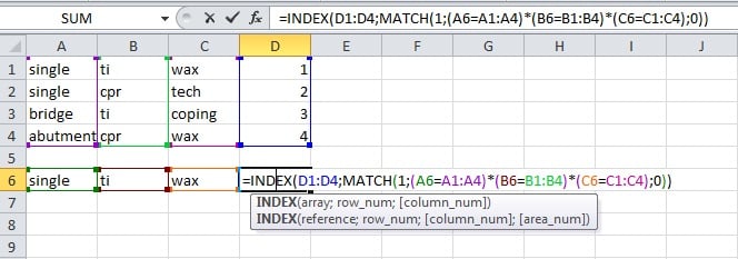
I'm trying to figure out how to do the following excel formula in Smartsheet, but I am having trouble with it. Can I get some help please ?

Basically what I need to do is match 3 different criteria (lookup 1 -3) with 3 different collumns(part 1 - 3) and when those match they have to give me the corresponding Time.

This is the excell formula : =INDEX(D1:D4;MATCH(1;(A6=A1:A4)*(B6=B1:B4)*(C6=C1:C4);0))

Find more posts tagged with

Healthcare

Comments

Taylor F

I tried to set up your example in Excel percisly the way that you have it outlined in your screenshot and I receive an error message.

INDEX has two required arguments. The first is the range of of the cells you would like to return. You have this with your D1:D4. The second is the row number which you are using MATCH to provide. This will work.

MATCH has two required arugments. The first is the value you are looking for. The second is a range you are looking for the value in.

(A6=A1:A4)*(B6=B1:B4)*(C6=C1:C4)

This is what you are using inte range argument of the MATCH. Breaking this up (without getting it to work in Excel) it appears that each section would produce a number of where row 6's value is located in the first four rows. Then it will multiple these numbers which would return an numeric value and not a range which MATCH is expecting in this argument.

This formula won't be able to be created in Smartsheet since MATCH isn't being provided a range.

If you have any questions or would like to dive into this further, please reach out to us submitting this form: https://help.smartsheet.com/contact and we will be happy to assist you.

-Taylor

Yannick Decock

@Taylor F

Thank you for the help!

The excell formula does work, Have you remembered to press Ctrl + Shift + Enter when using the formulae ? else it will not work and give you an error.

Either way I have managed to solve this problem in another way.

I Sum up all input into one big String value, then compare that to a database with all possible string value's and corresponding needed value as output.

Anyways, thanks again for hte help!

jryan

Yannick,

I'm trying to do the same thing. Can you share your solution?

Wilbsguy

I know this is old but hopefully this helps anyone else that wants this. What you want is another index formula within the match formula. So an index-match-index formula.

=INDEX(Time1:Time9, MATCH(1, INDEX(([lookup 1]1 = [part 1]1:[part 1]9)* ([lookup 2]1 = [part 2]1:[part 2]9)* ([lookup 3]1 = [part 3]1:[part 3]9)),0,1), 0))

Wilbsguy

I know it has been a while but if you still need something, I gave an answer. Let me know if you have any questions on it.

Hi All, Tacking onto the end of someone else's issue with my own...

I'm trying to make the formula above work with reference sheets:

=INDEX({Budget Day Rate}, MATCH(1, INDEX((Loc9 = {Budget Loc}) * ([Column3]9 = {Budget Role})), 0, 1), 0)

The above returns #INCORRECT ARGUMENT SET

Have also Tried:

=INDEX({Budget Day Rate}, MATCH(1, (Loc7 = {Budget Loc}) * ([Column3]7 = {Budget Role}), 0))

The above returns #INVALID OPERATION

{Budget Day Rate} = The day rate column in a rate card sheet

{Budget Loc} = The Location Column "UK" "US" etc

{Budget Role} = Column with Job title

My aim is to return the value from the "day rate column" If the Location and Job Title Match. A US Project Manager may earn a higher day rate than a UK Project Manager on the rate card. Any input on this would be amazing!

Andrée Starå

Hi,

You could maybe use a JOIN function to get the values together and only match that.

Would that work?

Can you describe your process in more detail and maybe share some screenshots? (Delete/replace any confidential/sensitive information before sharing) That would make it easier to help.

Have a fantastic weekend!

Best,

Andrée Starå

Workflow Consultant @ Get Done Consulting

Hi Andree,

Please see attached screen shot. If you're interested the sheets are in the shared workspace I created for you the other day for the checkbox formula Q I have elsewhere :-)

Basically, If Loc cell and Job Title cell in the same row, both match the respective value in the same row on the reference sheet (or lookup table) then I want to return the value in the third column of the reference sheet.

Ref Sheet, "Project Manager" in the "UK" day rate is "£10". In my budget sheet I want to return the value of "£10" in the "Day Rate" column if the "Loc" and "Job Title" match the values on the Rate card.

Thanks for looking!! :-)

Screenshot 2019-07-05 at 15.53.07.png

Andrée Starå

Thanks!

I'll take a look and get back to you! (for both)

Thank you!

FYI - I had previously asked my question in it's own thread: https://community.smartsheet.com/discussion/matching-multiple-values-multiple-columns-linked-sheet-fill-cell-content-third-column#comment-184841

Just managed to make the following do what I need:

=JOIN(COLLECT({Budget Day Rate}, {Budget Loc}, Loc@row, {Budget Role}, [Job Title]@row))

Andrée Starå

Excellent!

One left!

Actually that doesn't work - it returns the value I want but I then can't do anything with it... It breaks the formula in the next Column. It also won't take "£" formatting etc.

Soooo Close...

Andrée Starå

Hi,

Did you get it working?

Have a fantastic day!

Best,

Andrée Starå

Workflow Consultant @ Get Done Consulting

Hi Andree,

I am able to pull the right value BUT there is an issue with the column at that point, it won't allow me to use "£" formatting or do anything with the output. Other cells also don't see the output as a number which means it can't be used in a "SUM" in a different cell.

I tried to cheat and created a new column that used ="other cell" but it clones the issue...

Thanks for checking in.

The long and short of it is, I wan't to match the day rate to the user based on Location/Job role. That I can now do... but the £ value day rate is not seen as a number value. This means I can't then multiply the users correct day rate against the total number of days worked to give me a total cost of that user.

If "Olly" is based in "UK" and his Job is "Project Manager" his day rate is "£10" I will get a value of "10" in the cell, I want to make that a £ value and then multiply it by the 20 days worked which gives a total cost for Olly for that month of £200