Lookup function in Countifs statement?

In my sheet I have a list of projects with various statuses and I need to do summary numbers by month and reduce the number of statuses to 2 (scheduled and unscheduled). I know how to do this if I use the Lookup function to populate a column with the converted statuses, then use Countifs to get the numbers for each month.

My question is, is there a way to do this in a single formula?

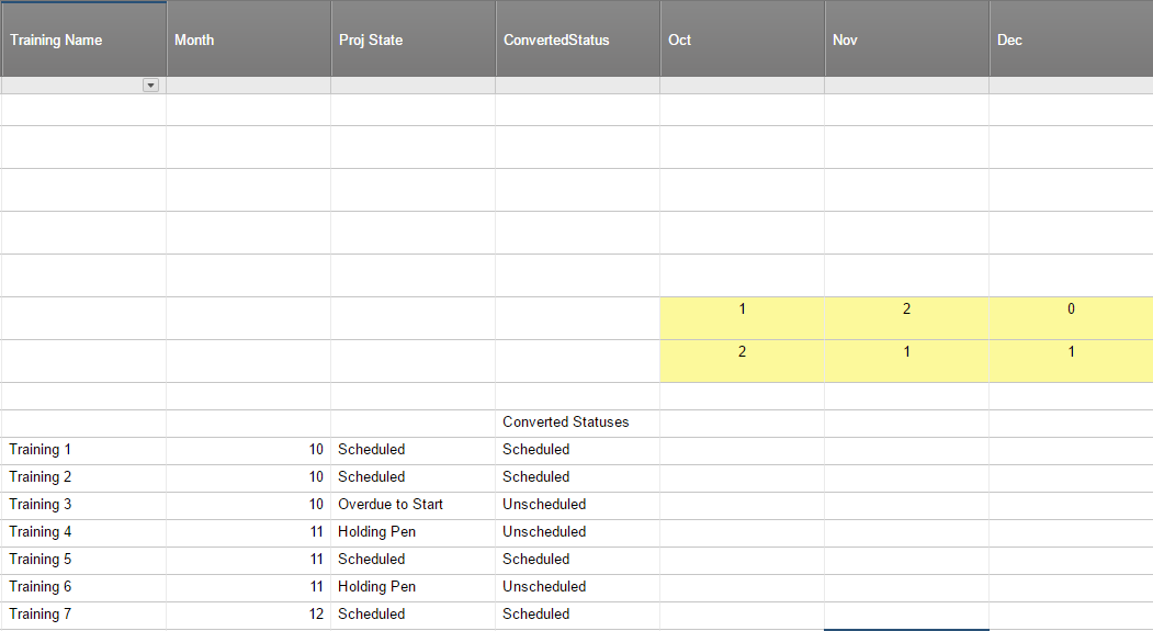
Here are samples of the formulas I'm using now:

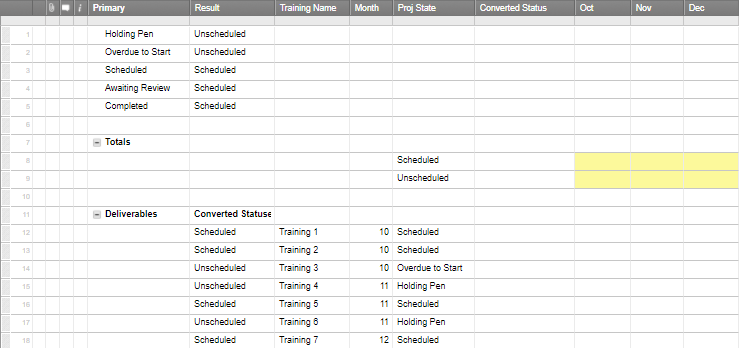
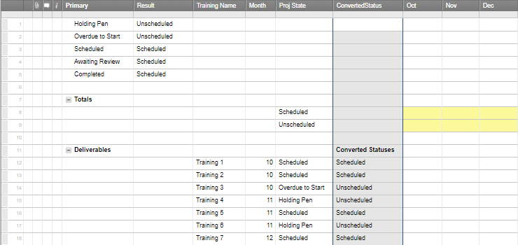
Converting a row in the Proj State column (with lots of statuses) to one of 2 statuses using a Lookup (this formula is in the ConvertedStatus column on every project row):

=LOOKUP([Proj State]12, Primary$1:Result$5, 2, false)

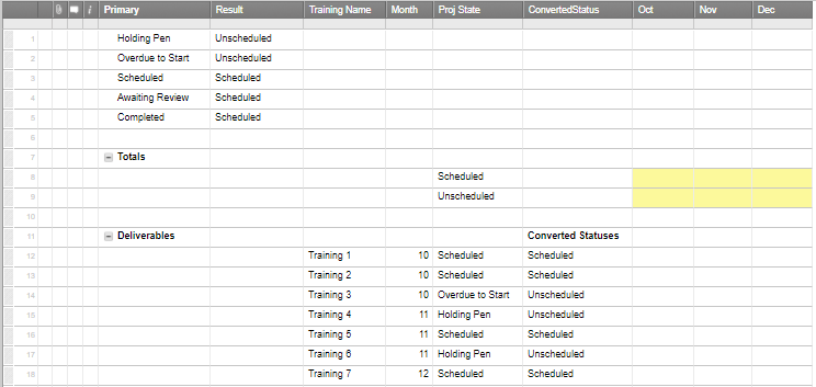
Calculating a monthly number in a range of cells using the converted status and month # - the sample is for October:

=COUNTIFS($Month12:$Month62, 10, $ConvertedStatus12:$ConvertedStatus62, ="Unscheduled")

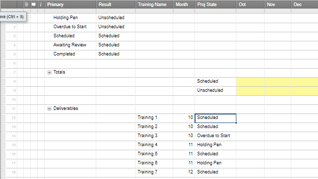
I'm trying to calculate the values in the yellow shaded columns in the screen shot.

Thanks!

Lookup Countifs formula help.png

Find more posts tagged with

Sheets

Formulas

Comments

Mike Andreas

Try these - keeping with the October example:

Top yellow cell:

=COUNTIFS($Month11:$Month17, 10, $ConvertedStatus11:$ConvertedStatus17, "Unscheduled")

Bottom yellow cell:

=COUNTIFS($Month11:$Month17, 10, $ConvertedStatus11:$ConvertedStatus17, "Scheduled")

I think all you needed to do was remove the last "=" that is before "Unscheduled".

Obviously you'll need to adjust the row numbers in the above equations. See this screenshot for verification.

Ron42na

Hmm...I looked at my post and realized it wasn't clear...

What I'm trying to do is avoid having to use the ConvertedStatus column...I'd like to do that determination on the fly by using the Lookup function in the Countifs formula.

Here's what I tried, but it gives me this error: #INCORRECT ARGUMENT SET

=COUNTIFS($Month12:$Month18, 10, LOOKUP([Proj State]12:[Proj State]18, Primary1:Result5, 2, false), "Unscheduled")

Mike Andreas

Are you trying to create an IF statement that counts the number of "Scheduled" and "Unscheduled" values, which by the way would be derived from the number of times other particular values appear? If so, this nested IF statement would rely heavily on two different OR functions.

Robert S.

Hello,

It sounds like you're looking to have these counts happen without having to use the "ConvertedStatus" column. In order to make this possible, you would also not be using the lookup table anymore. It also requires a longer formula.

Since we know what values mean both "Scheduled" and "Unscheduled" in the "Proj State" column, you can write your COUNTIFS formulas to look for these values instead. Since there are multiple values, we would want to write a formula that says "Count rows where the month column is 10, and the Proj State column is EITHER Holding Pen OR Overdue to Start" to get the equivalent of "Unscheduled". Since a COUNTIFS formula is inherintly an AND statement, we can't just use the OR function. Instead we would created one COUNTIFS statement for each Proj State value, and add them together. This is what the formula would look like for October Unscheduled:

=COUNTIFS(CHILDREN(Month11), 10, CHILDREN([Proj State]11), "Holding Pen") + COUNTIFS(CHILDREN(Month11), 10, CHILDREN([Proj State]11), "Overdue to Start")

You'll also notice that I replaced the cell ranges with the CHILDREN function. This is possible because the rows that contain the data are indented under row 11. This range will include all new rows that are added and indented under row 11. If you'd prefer to just use a normal cell range reference like you currently are, you can replace CHILDREN(Month11) with your Month column cell range, and CHILDREN([Proj State]11) with your Proj State column cell range.