Best Of

Prior to beginning my career, I had a completely different plan for my life. I had been studying Finance in hopes to obtain a corporate finance job for the retail company I worked for at the time. As the company changed, so did its culture, and I found myself looking for a fresh start and new challenge. Early in the morning, I had applied for a role at another company in which the job posting mentioned "security" and I figured that given my work history in retail and having dabbled in some work with loss prevention before, it might be a good fit. Later that morning, a recruiter reached out to me and offered me an interview within Assets Protection at a retail store. This was outside of my comfort zone, because I felt that I was not an "expert" in the field, and questioned why they'd want someone like me who didn't have the direct 1:1 experience.

Regardless, I took a leap of faith and decided to interview for the role and put my misgivings aside. I wound up getting the job, with a higher title/role than I had even originally applied for. Within 3 years of working Assets Protection in a retail store, I wanted to make more of an impact beyond my 4 walls, and help shape strategy. This is when I took my second big leap of faith and moved halfway across the country during Covid for an entry-level corporate role, my first white collar job. Even though it was an entry-level role and I was overqualified, I just wanted to get my foot in the door and have the opportunity to prove myself.

5 years have passed since then and I am very fortunate to have been promoted several times. I genuinely enjoy what I do, and wake up every day looking forward to making an impact and fulfilling my goal from years ago about helping shape strategy. I've been exposed to amazing leaders, mentors, and opportunities that I would never have dreamt of before. Looking back, I'm glad I did one thing - take a leap of faith. While the unknown can be frightening and full of uncertainty, I continually shocked myself with how resilient that I was.

For those uncertain in their career journey right now, take that leap of faith. You may surprise yourself with how adaptable you are, and how many opportunities you can seize. You've gotten to where you are because of who you are - trust in yourself and bet on yourself, because that'll always be a winning ticket.

My career was initially "forced" on me. Haha. I had just gotten transferred to another department that had more room for success when the company I was working for brought on Smartsheet as a solution.

My VP at the time told me that since I hadn't really learned the new position yet, I was going to take the lead on Smartsheet. Initially I was pretty frustrated as it was taking away from what I thought was a career move.

But… I was raised so that if I am going to do a job, I am going to do it right whether I liked it or not. So I dove in headfirst into Smartsheet learning everything that I could hoping that I could quickly move it off my plate and shift my focus back to where it belonged based on my new department.

Part of learning involved interacting here in the Community. Eventually some of my posts caught the attention of someone who owns a Smartsheet consulting company. One thing led to another, and here I am making a career of building Smartsheet solutions full time (which I now love to do).

I've noticed a few people asking for Speedometer Charts in Smartsheet, so I figured I would go ahead and publish this solution that I developed. It was some years ago, so there may be better ways and / or more efficient formulas, but this should at least help get everyone started…

A few notes to kick things off…

This solution has been built so that the percentages for each of the three colors is variable.

The indicator width is also variable.

Because we had to get a bit creative, we have to use our own legend and series labels. Since we have to build our own, I figured it wouldn't hurt to get creative with these as well. We can use a section in the underlying sheet with some formulas and conditional formatting to make them more flexible.

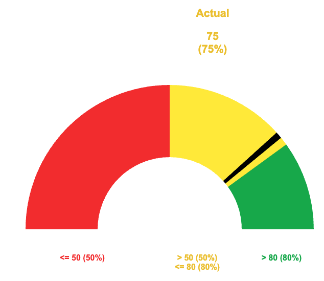
Singe the image above is static, I wanted to include that the indicator does move back and forth within the various colored sections to help visualize where within that section you really are.

This allows you to see if you are (for example) towards the lower end of yellow and in danger of going into the red or if you are in the higher end of yellow and almost into the green as opposed to just "yellow".

Basics:

There are three assets in total. A dashboard to display the chart and a sheet to format the data for the chart. These two are the focus of this thread.

The third asset will be your underlying data, but we aren't going to dive into that as there are too many different ways to collect your source data.

Below will be the details as well as screenshots for both the formatting sheet and the dashboard.

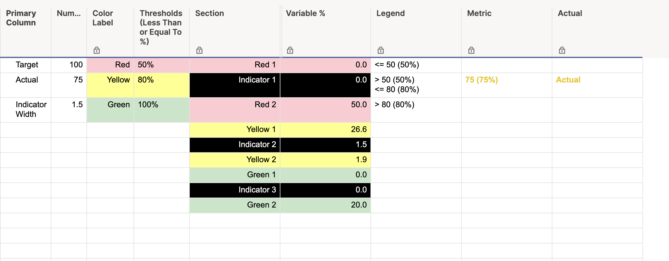
Formatting Sheet:

[Primary Column]:

NOTE: All rows in this column are manually entered.

Row 1: "Target"

Row 2: "Actual"

Row 3: "Indicator Width"

[Numbers]:

Row 1: Enter your target number. This number should be equivalent to your "100%" goal.

Row 2: This could be a cell link, a formula with a cross sheet reference, or even manually entered. This is going to be your "Actual" that is represented by the indicator in the chart.

Row 3: This is a manually entered number that indicates how wide you want the indicator in your chart. Lower numbers produce a thinner indicator, and larger numbers produce a thicker indicator. In the snippet above, the indicator width is 1.5.

[Color Label]:

NOTE: All rows in this column are manually entered.

Row 1: "Red" manually entered.

Row 2: "Yellow" manually entered.

Row 3: "Green" manually entered.

[Thresholds (Less Than or Equal To %)]:

NOTE: This column is formatted to show percentages.

Row 1: This will be the maximum percentage that would be considered "Red". For example, if you enter 50%, anything from 0% to 50% will have the indicator somewhere in the red section.

Row 2: This will be the maximum percentage that would be considered "Yellow". Using the example for Row 1, if you enter 80% here, anything above 50% but below 80% will have the indicator somewhere in the yellow section.

Row 3: 100% manually entered.

[Section]:

NOTE: All rows in this column are manually entered.

Row 1: "Red 1"

Row 2: "Indicator 1"

Row 3: "Red 2"

Row 4: "Yellow 1"

Row 5: "Indicator 2"

Row 6: "Yellow 2"

Row 7: "Green 1"

Row 8: "Indicator 3"

Row 9: "Green 2"

[Variable %]:

NOTE: All rows in this column are individual formulas.

Row 1:

=IF(Numbers2 > Numbers@row * [Thresholds (Less Than or Equal To %)]1, 0, (Numbers1 * [Thresholds (Less Than or Equal To %)]1) - ((Numbers1 * [Thresholds (Less Than or Equal To %)]1) - Numbers2) - Numbers3) + 0.00001

Row 2:

=IF(Numbers2 <= Numbers1 * [Thresholds (Less Than or Equal To %)]1, Numbers1 * (Numbers3 / 100), 0) + 0.00001

Row 3:

=IF(Numbers2 > Numbers1 * [Thresholds (Less Than or Equal To %)]1, Numbers1 * [Thresholds (Less Than or Equal To %)]1, (Numbers1 * [Thresholds (Less Than or Equal To %)]1) - Numbers2) + 0.00001

Row 4:

=IF(AND(Numbers2 < Numbers1 * [Thresholds (Less Than or Equal To %)]2, Numbers2 > Numbers1 * [Thresholds (Less Than or Equal To %)]1), (Numbers2 / (Numbers1 * [Thresholds (Less Than or Equal To %)]2)) * (Numbers1 * ([Thresholds (Less Than or Equal To %)]2 - [Thresholds (Less Than or Equal To %)]1)) - Numbers3, 0) + 0.00001

Row 5:

=IF(AND(Numbers2 <= Numbers1 * [Thresholds (Less Than or Equal To %)]2, Numbers2 > Numbers1 * [Thresholds (Less Than or Equal To %)]1), Numbers1 * (Numbers3 / 100), 0) + 0.00001

Row 6:

=IF(AND(Numbers2 < Numbers1 * [Thresholds (Less Than or Equal To %)]2, Numbers2 > Numbers1 * [Thresholds (Less Than or Equal To %)]1), (Numbers1 * ([Thresholds (Less Than or Equal To %)]2 - [Thresholds (Less Than or Equal To %)]1)) - ((Numbers2 / (Numbers1 * [Thresholds (Less Than or Equal To %)]2)) * (Numbers1 * ([Thresholds (Less Than or Equal To %)]2 - [Thresholds (Less Than or Equal To %)]1))), Numbers1 * ([Thresholds (Less Than or Equal To %)]2 - [Thresholds (Less Than or Equal To %)]1)) + 0.00001

Row 7:

=IF(Numbers2 > Numbers1 * [Thresholds (Less Than or Equal To %)]2, MIN((Numbers1 * ([Thresholds (Less Than or Equal To %)]3 - [Thresholds (Less Than or Equal To %)]2)) - (Numbers1 - Numbers2), Numbers1) - Numbers3, 0) + 0.00001

Row 8:

=IF(Numbers2 > Numbers1 * [Thresholds (Less Than or Equal To %)]2, Numbers1 * (Numbers3 / 100), 0) + 0.00001

Row 9:

=IF(Numbers2 >= Numbers1, 0, IF(Numbers2 > Numbers1 * [Thresholds (Less Than or Equal To %)]2, (Numbers1 * ([Thresholds (Less Than or Equal To %)]3 - [Thresholds (Less Than or Equal To %)]2)) - ((Numbers1 * ([Thresholds (Less Than or Equal To %)]3 - [Thresholds (Less Than or Equal To %)]2)) - (Numbers1 - Numbers2)), Numbers1 - (Numbers1 * [Thresholds (Less Than or Equal To %)]2))) + 0.00001

[Legend]:

NOTE: All rows in this column are individual formulas.

Row 1:

="<= " + ROUND((Numbers1 * [Thresholds (Less Than or Equal To %)]@row)) + " (" + ROUND([Thresholds (Less Than or Equal To %)]@row * 100) + "%)"

Row 2:

="> " + ROUND(Numbers1 * [Thresholds (Less Than or Equal To %)]1) + " (" + ROUND([Thresholds (Less Than or Equal To %)]1 * 100) + "%)" + CHAR(10) + "<= " + ROUND((Numbers1 * [Thresholds (Less Than or Equal To %)]2)) + " (" + ROUND([Thresholds (Less Than or Equal To %)]@row * 100) + "%)"

Row 3:

="> " + ROUND((Numbers1 * [Thresholds (Less Than or Equal To %)]2)) + " (" + ROUND([Thresholds (Less Than or Equal To %)]2 * 100) + "%)"

[Metric]:

NOTE: All rows in this column are individual formulas.

Row 1:

=IF(Numbers2 <= Numbers1 * [Thresholds (Less Than or Equal To %)]1, Numbers2 + " (" + ROUND(Numbers2 / Numbers1, 2) * 100 + "%)", 0)

Row 2:

=IF(AND(Numbers2 > Numbers1 * [Thresholds (Less Than or Equal To %)]1, Numbers2 <= Numbers1 * [Thresholds (Less Than or Equal To %)]2), Numbers2 + " (" + ROUND(Numbers2 / Numbers1, 2) * 100 + "%)", 0)

Row 3:

=IF(Numbers2 > Numbers1 * [Thresholds (Less Than or Equal To %)]2, Numbers2 + " (" + ROUND(Numbers2 / Numbers1, 2) * 100 + "%)", 0)

[Actual]:

NOTE: All rows in this column are manually entered.

Row 1, Row 2, and Row 3 all have the word "Actual" anually entered.

Conditional Formatting:

NOTE: I wasn't able to show it in the screenshot, but each rule is applied to the [Metric] and [Actual] columns.

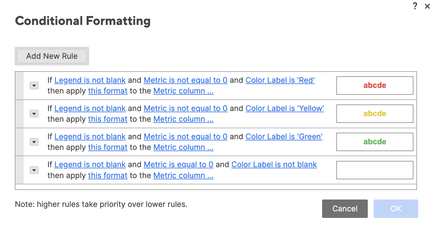
Screenshot of the formatting sheet:

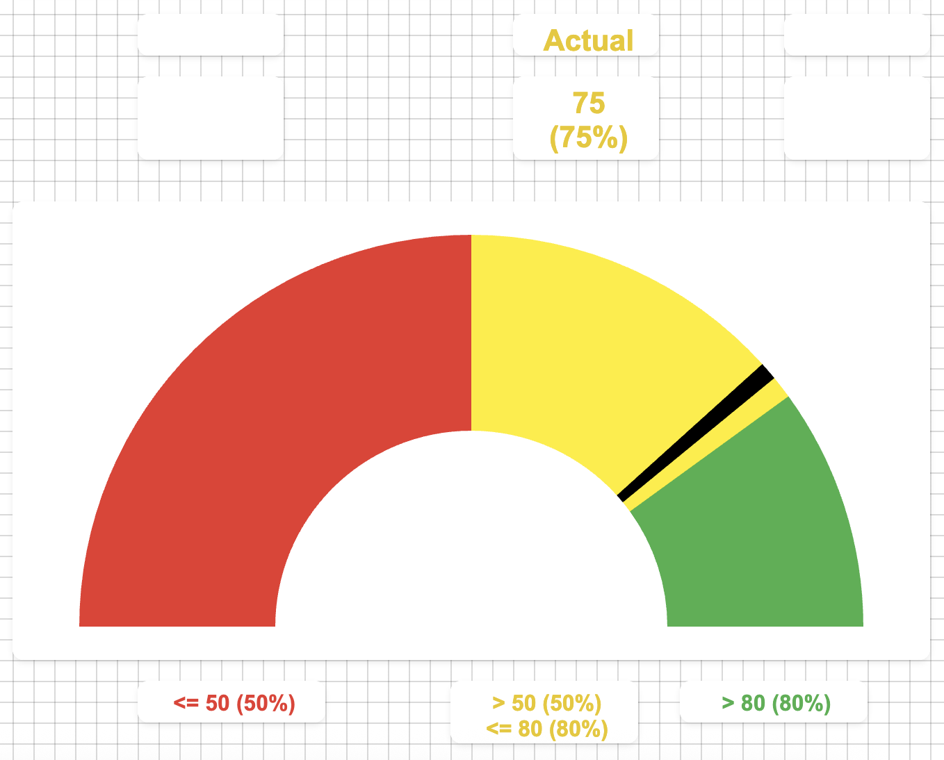
Dashboard:

You can use your own judgement for the sizes of each widget, but the general idea here is that we use individual metrics widgets to display the actuals and the "legend", and we use a half-donut chart for the "speedometer" portion.

You can see in the below screenshot how each of the widgets are laid out. I have the "Actuals" going across the top relatively in line with each of their colored sections, and the legend is metrics widgets across the bottom also in line with each of the colored sections.

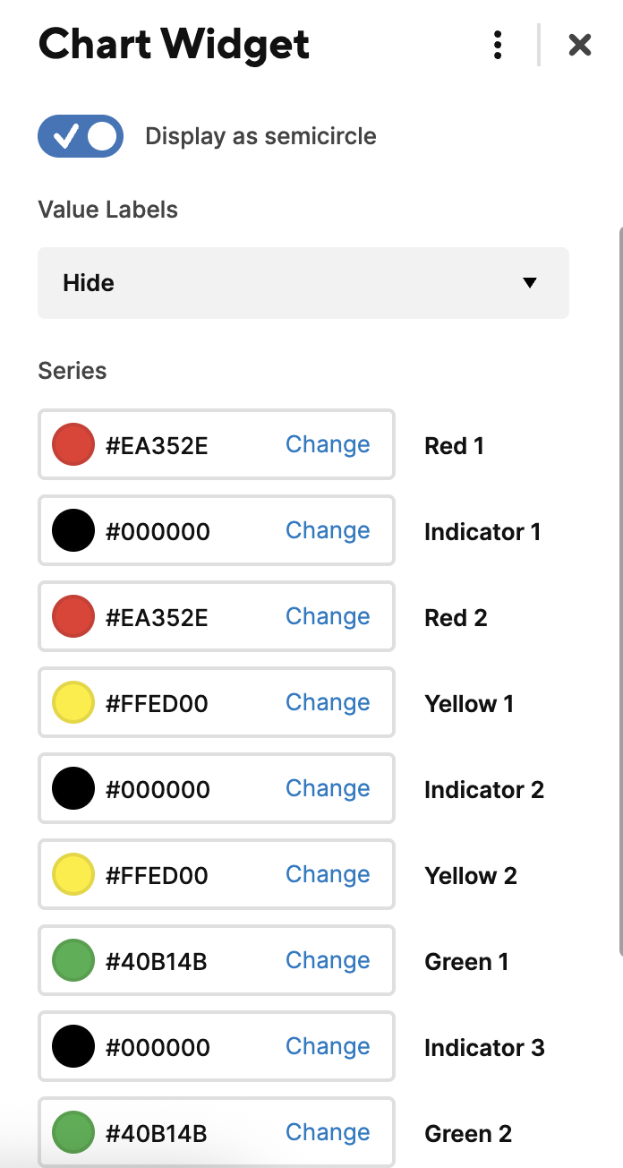
The "star of the show" here though is the speedometer chart. When we select the data for this, we select rows 1 through 9 of both the [Section] column and the [Variable %] column. I will provide a separate snippet of the chart series to show what colors were selected for the above.

Widget Layout:

Series: