Maximum Concurrent Tasks

Alkards85 · 02/20/25

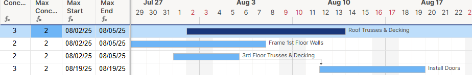
Working with a multi-family developer building multiple apartment buildings on the same project. Trying to get in front of bottlenecks in the schedule where we're expecting multiple crews in multiple buildings and end up short staffing or over staffing. For instance, Row 58 the Framer should be starting Task "Wall Framing" on 7/14/25.

However, I know this framer has multiple tasks across the project by viewing in Timeline:

I would like a formula in the Grid View to fill the "Maximum Concurrent Tasks" cell to return a value of "3" in this instance. That way I can conditionally format to call out when our schedule is overallocated. For instance in the following clip my schedule is calling for 6 crews to be on site for a stretch.

I don't believe I can do this with resource management because I don't want to require all our subcontractors to be registered users on our system.

jmyzk_cloudsmart_jp · 02/21/25

Hi @Alkards85

The COUNTIF formula will count all tasks where:

Their Start Date is before or on the End Date of the current task.
AND
Their End Date is after or on the Start Date of the current task.

=COUNTIFS([Start Date]:[Start Date], <=[End Date]@row, [End Date]:[End Date], >=[Start Date]@row, [Assigned To]:[Assigned To], [Assigned To]@row) - 1

Since the formula also counts the current row, it subtracts 1 to get concurrent tasks other than itself.

https://app.smartsheet.com/b/publish?EQBCT=7b10ede926104f94a4835a20496df75b (Link to the published demo sheet. You can change the Select row to see how the formula works.)

How to use this sheet

Look for the task with many concurrent tasks, such as the task in the second row. (There are three concurrent tasks.)
Check the Select column.
Overlapped tasks will be shown with conditional formatting.
Reconsider and update the assignments or schedule to lessen the overlap.
Create reports filtered by [Assigned To] value for your subcontractors or share the sheet filters (*).

Note: Overlap formula

=IFERROR(AND([Start Date]@row <= [Selected End Date]#, [End Date]@row >= [Selected Start Date]#, [Assigned To]@row = [Selected Assinged To]#), "")

Note: Summary Field formulas

[Selected Start Date]#=IFERROR(INDEX(COLLECT([Start Date]:[Start Date], Select:Select, true), 1), "")
[Selected End Date]#=IFERROR(INDEX(COLLECT([End Date]:[End Date], Select:Select, true), 1), "")
[Selected Assigned To]#=IFERROR(INDEX(COLLECT([Assigned To]:[Assigned To], Select:Select, true), 1), "")

(*) Sheet filtered by Framer 2.

Alkards85 · 02/21/25

Most of this looks great and the quick response is awesome!

Here's what I'm still missing:

The first couple pictures in my example the framer is starting wall framing on one building, that will take him 7 days. But the other concurrent tasks during that time are shorter durations completed by separate crews. So I can realistically run that 7 days with only 3 crews. That's where I need some version of MAX in the formula that would return "3" into that task. Since at most during this timeframe 7/14-7/22 I would need is 3 crews on site on that Wednesday and Thursday.

jmyzk_cloudsmart_jp · 02/22/25

Hi @Alkards85

It is pretty interesting to learn about real-world needs!

Below is the updated demo solution that takes into your requirements.

https://app.smartsheet.com/b/publish?EQBCT=cfc51e1994a947f8b94ca0353904fc57

As you can see, the selected task has three overlaps, but the maximum of two overlaps will happen on August 19, 2025.

I used this approach to count the maximum number.

Get each date of the task, starting from the Start Date and ending at the End Date.
For each date, check for overlaps with other tasks that contain the date in their task range.
1. For example, first check if the Start Date, 08/12/25, has any overlaps.
2. Then, the next day, 08/13/25, and so on, until the End Date, 08/19/25.
Then, count the number of such tasks.
Finally, get the maximum number of the counts.

So, I first added 20 helper columns, [D1] to [D20], assuming 20 dates would be enough for most of the task.

As you can see, the hepper columns populate dates within the [Start Date] and [End Date] ranges.

I used the following pattern of the formula;

[D1] =[Start Date]@row
[D2] =IF([D1]@row + 1 <= [End Date]@row, [D1]@row + 1)
[D3] =IF([D2]@row + 1 <= [End Date]@row, [D2]@row + 1)
…….
[D20] =IF([D19]@row + 1 <= [End Date]@row, [D19]@row + 1)

Second, I added 20 helper columns, [C1] to [C20], to populate the number of overlap tasks, including itself, on the corresponding date. For example, [C1] will populate the number of overlaps on [D1].

[C1] =COUNTIFS([Start Date]:[Start Date], <=[D1]@row, [End Date]:[End Date], >=[D1]@row, [Assigned To]:[Assigned To], [Assigned To]@row)

[C2] =COUNTIFS([Start Date]:[Start Date], <=[D2]@row, [End Date]:[End Date], >=[D2]@row, [Assigned To]:[Assigned To], [Assigned To]@row)
…….

[C20] =COUNTIFS([Start Date]:[Start Date], <=[D20]@row, [End Date]:[End Date], >=[D20]@row, [Assigned To]:[Assigned To], [Assigned To]@row)

Finally, I used the following to calculate the maximum number.

[Max Concurrent] =MAX([C1]@row:[C20]@row) - 1

As a bonus attempt, I created those formulas to show the start and end dates of the maximum overlap dates. For example, the maximum overlap for the Roof Trusees & Decking tasks starts on August 2 and ends on August 5.

[Max Start] =INDEX([D1]@row:[D20]@row, 1, MATCH([Max Concurrent]@row + 1, [C1]@row:[C20]@row, 0))
[Max End] =INDEX([D1]@row:[D20]@row, 1, MATCH([Max Concurrent]@row + 1, [C1]@row:[C20]@row, 0) + COUNTIF([C1]@row:[C20]@row, [Max Concurrent]@row + 1) - 1)

I created those helper columns using the proprietary API tool, as adding these many columns and formulas is time-consuming.
If you find replicating those helper columns and formulas tricky, please get in touch with me for the sheet share or any other help. (My email address is on the profile page.)

Alkards85 · 03/05/25

It's been a minute since I've been able to circle back to this, and it was working great. However, now I'm getting the cell references over 25M error. I can't say I understand what I've read regarding this error, but it seems like my row count of ~1400 tasks is multiplying the C1-D20 columns exponentially and putting me over this limit. Any suggestions, or should I just chalk this up as not possible?

jmyzk_cloudsmart_jp · 03/06/25

Hi @Alkards85

It looks like the "Too Many Cells Referenced" error you’re experiencing is indeed due to the exponential growth of cell references, especially from the [C1] to [C20] columns that use COUNTIFS with column-wide references (column:column). When your sheet has ~1400 tasks, the cumulative cell references can easily exceed the 25M limit.

I have updated the formulas to reduce column references significantly while achieving the same outcome to address this. Here's an explanation of the improved approach:

https://app.smartsheet.com/b/publish?EQBCT=78ca013cc45445218bbd988777699811

Formulas

[Max Concurrent] =MAX([C1]@row:[C20]@row)
[R1]to[R4] gets the row number of tasks which overlaps for a Assigned To
[R1] =IFERROR(INDEX(COLLECT(Row:Row, Row:Row, <>Row@row, [Assigned To]:[Assigned To], [Assigned To]@row, Start:Start, <=End@row, End:End, >=Start@row), 1), "") ….
[R4] =IFERROR(INDEX(COLLECT(Row:Row, Row:Row, <>Row@row, [Assigned To]:[Assigned To], [Assigned To]@row, Start:Start, <=End@row, End:End, >=Start@row), 4), "")
[S1]to[S4] and [E1]to[E4] gets the start date and end dates of those overlapping tasks.
[S1] =IF(ISNUMBER([R1]@row), INDEX(Start:Start, [R1]@row)) ….
[S4] =IF(ISNUMBER([R4]@row), INDEX(Start:Start, [R4]@row))
[E1] =IF(ISNUMBER([R1]@row), INDEX(End:End, [R1]@row))
….
[E4] =IF(ISNUMBER([R4]@row), INDEX(End:End, [R4]@row))
[C1] to [C20] counts the overlapping task for [D1] to [D2], using the above [S1]to[S4]and[E1]to[E4]
[C1] =IF(ISDATE([D1]@row), IF(AND([S1]@row <= [D1]@row, [E1]@row >= [D1]@row), 1, 0) + IF(AND([S2]@row <= [D1]@row, [E2]@row >= [D1]@row), 1, 0) + IF(AND([S3]@row <= [D1]@row, [E3]@row >= [D1]@row), 1, 0) + IF(AND([S4]@row <= [D1]@row, [E4]@row >= [D1]@row), 1, 0)) ….
(readable version)
[C20] =IF(ISDATE([D20]@row),
IF(AND([S1]@row <= [D20]@row, [E1]@row >= [D20]@row), 1, 0) +
IF(AND([S2]@row <= [D20]@row, [E2]@row >= [D20]@row), 1, 0) +
IF(AND([S3]@row <= [D20]@row, [E3]@row >= [D20]@row), 1, 0) +
IF(AND([S4]@row <= [D20]@row, [E4]@row >= [D20]@row), 1, 0))
[D1]to[D20] populates dates witin a task's duration
[D1] =Start@row …

[D20] =IF([D19]@row + 1 <= End@row, [D19]@row + 1)

Key Improvements in the Updated Formulas

Significant Reduction in Cell References
- Previous Method:
  [C1] to [C20] used COUNTIFS with [Start Date]:[Start Date], [End Date]:[End Date], and [Assigned To]:[Assigned To], causing exponential growth in references. For a sheet with 1400 rows, this approach generated approximately 117,600,000 references in total.
- Updated Method:
  Instead of referencing entire columns, the new formulas use COLLECT and INDEX to extract up to 4 overlapping tasks based on the same [Assigned To] value. By referencing only [S1] to [S4] and [E1] to [E4] for checking overlaps, the total cell references are reduced to about 224,000 references.
- Total Reduction: This change reduces cell references by about 117,376,000 (≈ 99.8% reduction), preventing the 25M error and improving performance significantly.
Extracting Up to 4 Overlapping Tasks Efficiently
- New Formula Approach: We now use [R1] to [R4] to store row numbers of up to 4 overlapping tasks using:
  [R1] =IFERROR(INDEX(COLLECT(Row:Row, Row:Row, <>Row@row, [Assigned To]:[Assigned To], [Assigned To]@row, Start:Start, <=End@row, End:End, >=Start@row), 1), "")
  - This formula finds the first overlapping task and stores its row number in [R1].
  - Similarly, [R2], [R3], and [R4] find and store the next three overlapping tasks.
Using Specific Date References Instead of Column References
- Previous Method: [C1] to [C20] used COUNTIFS with column references like [Start Date]:[Start Date] to check overlaps.
- Updated Method: We now store the start and end dates of the overlapping tasks directly in [S1] to [S4] (Start Dates) and [E1] to [E4] (End Dates) using:
  [S1] =IF(ISNUMBER([R1]@row), INDEX(Start:Start, [R1]@row))
  [E1] =IF(ISNUMBER([R1]@row), INDEX(End:End, [R1]@row))
  - This eliminates the need to reference entire date columns repeatedly.
  - Only the dates of the overlapping tasks are referenced, reducing the total cell reference count dramatically.
Optimized Overlap Counting with Limited References
- Previous Approach:
  [C1] =COUNTIFS([Start Date]:[Start Date], <=[D1]@row, [End Date]:[End Date], >=[D1]@row, [Assigned To]:[Assigned To], [Assigned To]@row)
  - This formula caused a massive increase in cell references due to full-column referencing combined with multiple conditions.
- New Approach:
  [C1] =IF(ISDATE([D1]@row), IF(AND([S1]@row <= [D1]@row, [E1]@row >= [D1]@row), 1, 0) + IF(AND([S2]@row <= [D1]@row, [E2]@row >= [D1]@row), 1, 0) + IF(AND([S3]@row <= [D1]@row, [E3]@row >= [D1]@row), 1, 0) + IF(AND([S4]@row <= [D1]@row, [E4]@row >= [D1]@row), 1, 0))
  - This formula checks overlaps only against the specific four tasks instead of the entire column.
  - By using [S1] to [S4] and [E1] to [E4], we limit the references to a maximum of 4 tasks per row.
Efficient Date Management
- The [D1] to [D20] columns that generate date sequences remain the same, but benefit from the reduced overhead caused by optimized [C1] to [C20] formulas.
- Since each date now checks overlap against a maximum of 4 specific tasks instead of entire columns, this part of the formula becomes significantly lighter.

Please let me know if you need further assistance implementing these changes or have more questions!

Alkards85 · 03/06/25

Working through updating it now. What is the difference between the Row and Row ID columns? I didn't see either of them listed in the formulas, but could pull the "Row" column formula from the sample sheet you sent.

Alkards85 · 03/06/25

After adding a "Row ID" column and just autonumbering I placed the formula in that you had for "Row", knowing it's pretty much 2 redundant columns. Once I updated the rest of the formulas and it looks like I'm still over the capability of Smartsheet:

jmyzk_cloudsmart_jp · 03/07/25

Hi @Alkards85

I further updated the solution to decrease the number of column references;

In the previous solution, the demo sheet's R1, R2, R3 and R4 each used the column reference like this;
- [R1] =IFERROR(INDEX(COLLECT(Row:Row, Row:Row, <>Row@row, [Assigned To]:[Assigned To], [Assigned To]@row, Start:Start, <=End@row, End:End, >=Start@row), 1), "") …
- [R4] =IFERROR(INDEX(COLLECT(Row:Row, Row:Row, <>Row@row, [Assigned To]:[Assigned To], [Assigned To]@row, Start:Start, <=End@row, End:End, >=Start@row), 4), "")
I created a text helper column [Rs] to reduce the number of column references.
- For example, in the image below, the 1408th row has [Rs] like 1404,1414,1416,1419,1422,1433, which means those are the row numbers of the tasks by Framer 2 which overlaps with the 1408th row's task.
Then, using the TEXT functions like FIND, MID, LEFT, RIGHT, I retrieved the R1 to R4, without using the column references.

Regarding the RowID (system auto number) vs Row (which used the MATCH function), RowID is used to get a unique value and MATCH is used to get the row number. This technique is sometimes used when users move the rows around, which changes the auto number RowID. However, the MATCH function uses column reference, RowID:RowID, which adds the column references.
So, I simply put number 1 to 1418 and further to decrease the column reference.

https://app.smartsheet.com/b/publish?EQBCT=ef35645ab7e843e79228cb3671ba5218

Sheet Summary Fields Column References

I have three column references in the Sheet Summary Fields: Start:Start, End:End and [Assigned To]:[Assigned To].
I use those to highlight the Gantt chart bar for easy reference. But, if you only want to know the max concurrent tasks, you can remove them, decreasing the number of column references.

Formulas

Below are the formulas. I listed all the formulas so that you can copy & paste.
Note: If you are not using the Gant Bar conditional formatting using the Sheet Summary fields, you do not need the [Ooverlap] column and its formula.

[Overlap] =IFERROR(AND(Start@row <= [Selected End Date]#, End@row >= [Selected Start Date]#, [Assigned To]@row = [Selected Assinged To]#), "")
[Max Concurrent] =MAX([C1]@row:[C20]@row)
[Rs] =JOIN(COLLECT(Row:Row, Row:Row, <>Row@row, [Assigned To]:[Assigned To], [Assigned To]@row, Start:Start, <=End@row, End:End, >=Start@row), ",")
[Concurrents] =IF(ISBLANK(Rs@row), 0, LEN(Rs@row) - LEN(SUBSTITUTE(Rs@row, ",", "")) + 1)
[F0] =0
[F1] =IF(Concurrents@row > 1, FIND(",", Rs@row))
[F2] =IF(Concurrents@row > 2, FIND(",", Rs@row, [F1]@row + 1))
[F3] =IF(Concurrents@row > 3, FIND(",", Rs@row, [F2]@row + 1))
[F4] =IF(Concurrents@row > 4, FIND(",", Rs@row, [F3]@row + 1))
[F5] =IF(Concurrents@row > 5, FIND(",", Rs@row, [F4]@row + 1))
[R1] =IF(Concurrents@row < 2, Rs@row, MID(Rs@row, [F0]@row + 1, [F1]@row - [F0]@row - 1))
[R2] =IF(Concurrents@row > 1, IF(Concurrents@row < 3, RIGHT(Rs@row, LEN(Rs@row) - [F1]@row), MID(Rs@row, [F1]@row + 1, [F2]@row - [F1]@row - 1)))
[R3] =IF(Concurrents@row > 2, IF(Concurrents@row < 4, RIGHT(Rs@row, LEN(Rs@row) - [F2]@row), MID(Rs@row, [F2]@row + 1, [F3]@row - [F2]@row - 1)))
[R4] =IF(Concurrents@row > 3, IF(Concurrents@row < 5, RIGHT(Rs@row, LEN(Rs@row) - [F3]@row), MID(Rs@row, [F3]@row + 1, [F4]@row - [F3]@row - 1)))
[R5] =IF(Concurrents@row > 4, IF(Concurrents@row < 6, RIGHT(Rs@row, LEN(Rs@row) - [F4]@row), MID(Rs@row, [F4]@row + 1, [F5]@row - [F4]@row - 1)))
[S1] =IF(ISBLANK([R1]@row), "", INDEX(Start:Start, VALUE([R1]@row)))
[S2] =IF(ISBLANK([R2]@row), "", INDEX(Start:Start, VALUE([R2]@row)))
[S3] =IF(ISBLANK([R3]@row), "", INDEX(Start:Start, VALUE([R3]@row)))
[S4] =IF(ISBLANK([R4]@row), "", INDEX(Start:Start, VALUE([R4]@row)))
[E1] =IF(ISBLANK([R1]@row), "", INDEX(End:End, VALUE([R1]@row)))
[E2] =IF(ISBLANK([R2]@row), "", INDEX(End:End, VALUE([R2]@row)))
[E3] =IF(ISBLANK([R3]@row), "", INDEX(End:End, VALUE([R3]@row)))
[E4] =IF(ISBLANK([R4]@row), "", INDEX(End:End, VALUE([R4]@row)))
[C1] =IF(ISDATE([D1]@row), IF(ISDATE([S1]@row), IF(AND([S1]@row <= [D1]@row, [E1]@row >= [D1]@row), 1, 0), 0) + IF(ISDATE([S2]@row), IF(AND([S2]@row <= [D1]@row, [E2]@row >= [D1]@row), 1, 0), 0) + IF(ISDATE([S3]@row), IF(AND([S3]@row <= [D1]@row, [E3]@row >= [D1]@row), 1, 0), 0) + IF(ISDATE([S4]@row), IF(AND([S4]@row <= [D1]@row, [E4]@row >= [D1]@row), 1, 0), 0))
[C2] =IF(ISDATE([D2]@row), IF(ISDATE([S1]@row), IF(AND([S1]@row <= [D2]@row, [E1]@row >= [D2]@row), 1, 0), 0) + IF(ISDATE([S2]@row), IF(AND([S2]@row <= [D2]@row, [E2]@row >= [D2]@row), 1, 0), 0) + IF(ISDATE([S3]@row), IF(AND([S3]@row <= [D2]@row, [E3]@row >= [D2]@row), 1, 0), 0) + IF(ISDATE([S4]@row), IF(AND([S4]@row <= [D2]@row, [E4]@row >= [D2]@row), 1, 0), 0))
[C3] =IF(ISDATE([D3]@row), IF(ISDATE([S1]@row), IF(AND([S1]@row <= [D3]@row, [E1]@row >= [D3]@row), 1, 0), 0) + IF(ISDATE([S2]@row), IF(AND([S2]@row <= [D3]@row, [E2]@row >= [D3]@row), 1, 0), 0) + IF(ISDATE([S3]@row), IF(AND([S3]@row <= [D3]@row, [E3]@row >= [D3]@row), 1, 0), 0) + IF(ISDATE([S4]@row), IF(AND([S4]@row <= [D3]@row, [E4]@row >= [D3]@row), 1, 0), 0))
[C4] =IF(ISDATE([D4]@row), IF(ISDATE([S1]@row), IF(AND([S1]@row <= [D4]@row, [E1]@row >= [D4]@row), 1, 0), 0) + IF(ISDATE([S2]@row), IF(AND([S2]@row <= [D4]@row, [E2]@row >= [D4]@row), 1, 0), 0) + IF(ISDATE([S3]@row), IF(AND([S3]@row <= [D4]@row, [E3]@row >= [D4]@row), 1, 0), 0) + IF(ISDATE([S4]@row), IF(AND([S4]@row <= [D4]@row, [E4]@row >= [D4]@row), 1, 0), 0))
[C5] =IF(ISDATE([D5]@row), IF(ISDATE([S1]@row), IF(AND([S1]@row <= [D5]@row, [E1]@row >= [D5]@row), 1, 0), 0) + IF(ISDATE([S2]@row), IF(AND([S2]@row <= [D5]@row, [E2]@row >= [D5]@row), 1, 0), 0) + IF(ISDATE([S3]@row), IF(AND([S3]@row <= [D5]@row, [E3]@row >= [D5]@row), 1, 0), 0) + IF(ISDATE([S4]@row), IF(AND([S4]@row <= [D5]@row, [E4]@row >= [D5]@row), 1, 0), 0))
[C6] =IF(ISDATE([D6]@row), IF(ISDATE([S1]@row), IF(AND([S1]@row <= [D6]@row, [E1]@row >= [D6]@row), 1, 0), 0) + IF(ISDATE([S2]@row), IF(AND([S2]@row <= [D6]@row, [E2]@row >= [D6]@row), 1, 0), 0) + IF(ISDATE([S3]@row), IF(AND([S3]@row <= [D6]@row, [E3]@row >= [D6]@row), 1, 0), 0) + IF(ISDATE([S4]@row), IF(AND([S4]@row <= [D6]@row, [E4]@row >= [D6]@row), 1, 0), 0))
[C7] =IF(ISDATE([D7]@row), IF(ISDATE([S1]@row), IF(AND([S1]@row <= [D7]@row, [E1]@row >= [D7]@row), 1, 0), 0) + IF(ISDATE([S2]@row), IF(AND([S2]@row <= [D7]@row, [E2]@row >= [D7]@row), 1, 0), 0) + IF(ISDATE([S3]@row), IF(AND([S3]@row <= [D7]@row, [E3]@row >= [D7]@row), 1, 0), 0) + IF(ISDATE([S4]@row), IF(AND([S4]@row <= [D7]@row, [E4]@row >= [D7]@row), 1, 0), 0))
[C8] =IF(ISDATE([D8]@row), IF(ISDATE([S1]@row), IF(AND([S1]@row <= [D8]@row, [E1]@row >= [D8]@row), 1, 0), 0) + IF(ISDATE([S2]@row), IF(AND([S2]@row <= [D8]@row, [E2]@row >= [D8]@row), 1, 0), 0) + IF(ISDATE([S3]@row), IF(AND([S3]@row <= [D8]@row, [E3]@row >= [D8]@row), 1, 0), 0) + IF(ISDATE([S4]@row), IF(AND([S4]@row <= [D8]@row, [E4]@row >= [D8]@row), 1, 0), 0))
[C9] =IF(ISDATE([D9]@row), IF(ISDATE([S1]@row), IF(AND([S1]@row <= [D9]@row, [E1]@row >= [D9]@row), 1, 0), 0) + IF(ISDATE([S2]@row), IF(AND([S2]@row <= [D9]@row, [E2]@row >= [D9]@row), 1, 0), 0) + IF(ISDATE([S3]@row), IF(AND([S3]@row <= [D9]@row, [E3]@row >= [D9]@row), 1, 0), 0) + IF(ISDATE([S4]@row), IF(AND([S4]@row <= [D9]@row, [E4]@row >= [D9]@row), 1, 0), 0))
[C10] =IF(ISDATE([D10]@row), IF(ISDATE([S1]@row), IF(AND([S1]@row <= [D10]@row, [E1]@row >= [D10]@row), 1, 0), 0) + IF(ISDATE([S2]@row), IF(AND([S2]@row <= [D10]@row, [E2]@row >= [D10]@row), 1, 0), 0) + IF(ISDATE([S3]@row), IF(AND([S3]@row <= [D10]@row, [E3]@row >= [D10]@row), 1, 0), 0) + IF(ISDATE([S4]@row), IF(AND([S4]@row <= [D10]@row, [E4]@row >= [D10]@row), 1, 0), 0))
[C11] =IF(ISDATE([D11]@row), IF(ISDATE([S1]@row), IF(AND([S1]@row <= [D11]@row, [E1]@row >= [D11]@row), 1, 0), 0) + IF(ISDATE([S2]@row), IF(AND([S2]@row <= [D11]@row, [E2]@row >= [D11]@row), 1, 0), 0) + IF(ISDATE([S3]@row), IF(AND([S3]@row <= [D11]@row, [E3]@row >= [D11]@row), 1, 0), 0) + IF(ISDATE([S4]@row), IF(AND([S4]@row <= [D11]@row, [E4]@row >= [D11]@row), 1, 0), 0))
[C12] =IF(ISDATE([D12]@row), IF(ISDATE([S1]@row), IF(AND([S1]@row <= [D12]@row, [E1]@row >= [D12]@row), 1, 0), 0) + IF(ISDATE([S2]@row), IF(AND([S2]@row <= [D12]@row, [E2]@row >= [D12]@row), 1, 0), 0) + IF(ISDATE([S3]@row), IF(AND([S3]@row <= [D12]@row, [E3]@row >= [D12]@row), 1, 0), 0) + IF(ISDATE([S4]@row), IF(AND([S4]@row <= [D12]@row, [E4]@row >= [D12]@row), 1, 0), 0))
[C13] =IF(ISDATE([D13]@row), IF(ISDATE([S1]@row), IF(AND([S1]@row <= [D13]@row, [E1]@row >= [D13]@row), 1, 0), 0) + IF(ISDATE([S2]@row), IF(AND([S2]@row <= [D13]@row, [E2]@row >= [D13]@row), 1, 0), 0) + IF(ISDATE([S3]@row), IF(AND([S3]@row <= [D13]@row, [E3]@row >= [D13]@row), 1, 0), 0) + IF(ISDATE([S4]@row), IF(AND([S4]@row <= [D13]@row, [E4]@row >= [D13]@row), 1, 0), 0))
[C14] =IF(ISDATE([D14]@row), IF(ISDATE([S1]@row), IF(AND([S1]@row <= [D14]@row, [E1]@row >= [D14]@row), 1, 0), 0) + IF(ISDATE([S2]@row), IF(AND([S2]@row <= [D14]@row, [E2]@row >= [D14]@row), 1, 0), 0) + IF(ISDATE([S3]@row), IF(AND([S3]@row <= [D14]@row, [E3]@row >= [D14]@row), 1, 0), 0) + IF(ISDATE([S4]@row), IF(AND([S4]@row <= [D14]@row, [E4]@row >= [D14]@row), 1, 0), 0))
[C15] =IF(ISDATE([D15]@row), IF(ISDATE([S1]@row), IF(AND([S1]@row <= [D15]@row, [E1]@row >= [D15]@row), 1, 0), 0) + IF(ISDATE([S2]@row), IF(AND([S2]@row <= [D15]@row, [E2]@row >= [D15]@row), 1, 0), 0) + IF(ISDATE([S3]@row), IF(AND([S3]@row <= [D15]@row, [E3]@row >= [D15]@row), 1, 0), 0) + IF(ISDATE([S4]@row), IF(AND([S4]@row <= [D15]@row, [E4]@row >= [D15]@row), 1, 0), 0))
[C16] =IF(ISDATE([D16]@row), IF(ISDATE([S1]@row), IF(AND([S1]@row <= [D16]@row, [E1]@row >= [D16]@row), 1, 0), 0) + IF(ISDATE([S2]@row), IF(AND([S2]@row <= [D16]@row, [E2]@row >= [D16]@row), 1, 0), 0) + IF(ISDATE([S3]@row), IF(AND([S3]@row <= [D16]@row, [E3]@row >= [D16]@row), 1, 0), 0) + IF(ISDATE([S4]@row), IF(AND([S4]@row <= [D16]@row, [E4]@row >= [D16]@row), 1, 0), 0))
[C17] =IF(ISDATE([D17]@row), IF(ISDATE([S1]@row), IF(AND([S1]@row <= [D17]@row, [E1]@row >= [D17]@row), 1, 0), 0) + IF(ISDATE([S2]@row), IF(AND([S2]@row <= [D17]@row, [E2]@row >= [D17]@row), 1, 0), 0) + IF(ISDATE([S3]@row), IF(AND([S3]@row <= [D17]@row, [E3]@row >= [D17]@row), 1, 0), 0) + IF(ISDATE([S4]@row), IF(AND([S4]@row <= [D17]@row, [E4]@row >= [D17]@row), 1, 0), 0))
[C18] =IF(ISDATE([D18]@row), IF(ISDATE([S1]@row), IF(AND([S1]@row <= [D18]@row, [E1]@row >= [D18]@row), 1, 0), 0) + IF(ISDATE([S2]@row), IF(AND([S2]@row <= [D18]@row, [E2]@row >= [D18]@row), 1, 0), 0) + IF(ISDATE([S3]@row), IF(AND([S3]@row <= [D18]@row, [E3]@row >= [D18]@row), 1, 0), 0) + IF(ISDATE([S4]@row), IF(AND([S4]@row <= [D18]@row, [E4]@row >= [D18]@row), 1, 0), 0))
[C19] =IF(ISDATE([D19]@row), IF(ISDATE([S1]@row), IF(AND([S1]@row <= [D19]@row, [E1]@row >= [D19]@row), 1, 0), 0) + IF(ISDATE([S2]@row), IF(AND([S2]@row <= [D19]@row, [E2]@row >= [D19]@row), 1, 0), 0) + IF(ISDATE([S3]@row), IF(AND([S3]@row <= [D19]@row, [E3]@row >= [D19]@row), 1, 0), 0) + IF(ISDATE([S4]@row), IF(AND([S4]@row <= [D19]@row, [E4]@row >= [D19]@row), 1, 0), 0))
[C20] =IF(ISDATE([D20]@row), IF(ISDATE([S1]@row), IF(AND([S1]@row <= [D20]@row, [E1]@row >= [D20]@row), 1, 0), 0) + IF(ISDATE([S2]@row), IF(AND([S2]@row <= [D20]@row, [E2]@row >= [D20]@row), 1, 0), 0) + IF(ISDATE([S3]@row), IF(AND([S3]@row <= [D20]@row, [E3]@row >= [D20]@row), 1, 0), 0) + IF(ISDATE([S4]@row), IF(AND([S4]@row <= [D20]@row, [E4]@row >= [D20]@row), 1, 0), 0))
[D1] =Start@row
[D2] =IF([D1]@row + 1 <= End@row, [D1]@row + 1)
[D3] =IF([D2]@row + 1 <= End@row, [D2]@row + 1)
[D4] =IF([D3]@row + 1 <= End@row, [D3]@row + 1)
[D5] =IF([D4]@row + 1 <= End@row, [D4]@row + 1)
[D6] =IF([D5]@row + 1 <= End@row, [D5]@row + 1)
[D7] =IF([D6]@row + 1 <= End@row, [D6]@row + 1)
[D8] =IF([D7]@row + 1 <= End@row, [D7]@row + 1)
[D9] =IF([D8]@row + 1 <= End@row, [D8]@row + 1)
[D10] =IF([D9]@row + 1 <= End@row, [D9]@row + 1)
[D11] =IF([D10]@row + 1 <= End@row, [D10]@row + 1)
[D12] =IF([D11]@row + 1 <= End@row, [D11]@row + 1)
[D13] =IF([D12]@row + 1 <= End@row, [D12]@row + 1)
[D14] =IF([D13]@row + 1 <= End@row, [D13]@row + 1)
[D15] =IF([D14]@row + 1 <= End@row, [D14]@row + 1)
[D16] =IF([D15]@row + 1 <= End@row, [D15]@row + 1)
[D17] =IF([D16]@row + 1 <= End@row, [D16]@row + 1)
[D18] =IF([D17]@row + 1 <= End@row, [D17]@row + 1)
[D19] =IF([D18]@row + 1 <= End@row, [D18]@row + 1)
[D20] =IF([D19]@row + 1 <= End@row, [D19]@row + 1)

Maximum Concurrent Tasks

Answers

Categories